Excel can automatically change the appearance of cells according to their values using Conditional Formatting. It is one of the simplest ways to make large spreadsheets easier to read and analyse. Microsoft supports conditional formatting in current Excel versions, including Microsoft 365 and Excel 2024.
Here are seven practical ways to use it.
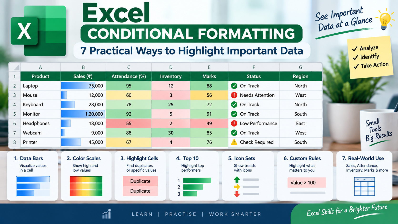
- Highlight important numbers Select your data and choose Home → Conditional Formatting → Highlight Cells Rules. You can highlight values greater than, less than, equal to or between selected numbers.
- Show high and low values with Color Scales Color scales use different shades to show whether values are relatively high, medium or low. This works well for marks, sales and performance data.
- Add Data Bars Data bars place a bar inside each cell. A larger number gets a longer bar, making comparisons easy without creating a chart.
- Use Icon Sets Icon sets can classify results using arrows, symbols or other indicators. They are useful for showing performance trends.
- Find Duplicate Values Choose Conditional Formatting → Highlight Cells Rules → Duplicate Values to quickly identify repeated entries. This is useful when cleaning customer lists or registration data.
- Highlight Top or Bottom Performers Use Top/Bottom Rules to highlight the top 10 items, bottom 10%, or another ranking. For example, you can identify your five highest-selling products.
- Create a custom rule For more control, choose New Rule and build a condition based on your own requirement.
Conditional formatting is especially useful in marksheets, attendance sheets, sales reports, inventory lists and dashboards.
The key is to use formatting to answer a question: What information should the reader notice first?
When used properly, conditional formatting turns a plain spreadsheet into a much more informative visual report.